R. A. Wood Associates QuickNews

Spectrum Analyzer Instrument Driver

LabVIEW Example - Spectrum Analyzer Instrument Driver

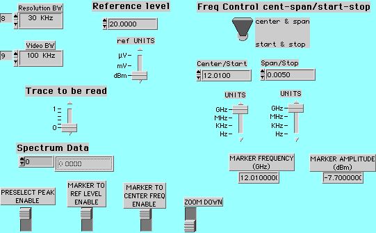
This LabVIEW panel shows an software controlled instrument driver that is utilized for HP Spectrum Analyzers. The software has been used on HP-8566B and HP-8593E Series Spectrum Analyzers. All front panel controls are translated to GPIB commands to control the equipment over a GPIB interface. The output readings are Marker Frequency and Marker Amplitude. Various options are included for locating and finding RF signals.

Tuning Station Example (Audible Feedback)

Tuning Station Example (Audible Feedback)

In this example an amplifier tuning station provides audible feedback to aid the technician in tuning the amplifier within its specified performance limits. The technician can tune the amplifier under a microscope, using the audio tones to indicate how close the device meets its specified performance window. The technician does not have to look up from his work to check an instrument panel to determine the results of his/her tuning.

R. A. Wood Associates can custom develop automated test software for your particular needs in your test station. We can provide and implement ideas to enhance your productivity.

Statistical Data Reduction and Analysis

Statistical Data Reduction and Analysis

R. A. Wood Associates Software can save valuable test and debug time by analyzing and summarizing large quantities of data. This example shows the result of taking 500 frequency readings from a Digital Frequency Discriminator (DFD) under low signal to noise ratio conditions. The DFD frequency error is plotted on the graph vs input frequency. The statistics of the frequency error are evaluated in the Test Summary and compared against the specifications. The test operator obtains immediate feedback from the results of the measurements.

User Friendly Test System Interface

User Friendly Test System Interface

The LabVIEW software developed by R. A. Wood Associates provides a user friendly interface to the automated test setup. The computer screen is the Test Panel, where input test parameters are entered or selected. Selection switches can be placed on the screen to control the hardware being tested.

After the test is completed, the output data is summarized, plotted, and printed out. Actual test data points can be stored in data files if needed.

Typical Automated Test Setup (Microwave Test)

Typical Automated Test Setup (Microwave Test)

This diagram shows a typical computer automated test setup. In this application, a microwave device is tested using microwave test equipment such as the signal generator, spectrum analyzer, and power meter. The digital I/O controller provides the logic controls for the Device Under Test while the logic analyzer reads digital information from the device.

The computer acts as the automated test controller. It controls the microwave test equipment to provide stimulus and measurements to and from the Device Under Test. Digital control is passed from the computer through the digital I/O board. Digital output data is passed from the logic analyzer to the computer.

The R. A. Wood Associates software will control the testing and analyze the measurements. Typical measurements may include gain, noise figure, gain compression, spurious signals, filter rejection and amplitude accuracy. The measured data is then summarized, eliminating the need for manual data reduction. Output data can be stored in data files for further analysis and evaluation.

Two Tone Third Order Output Intercept Point Measurements

Two Tone Third Order Output Intercept Point Measurements

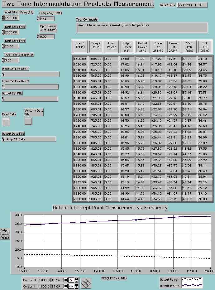
This LabVIEW panel shows the results of computer automated Two-Tone Third Order Output Intercept Point measurements for a PCS band RF amplifier. Measurements were performed using two programmable signal generators and a spectrum analyzer. A power meter was used to calibrate the input and output cables and connectors, and the spectrum analyzer amplitude readings. This panel design is tailored toward an "engineering evaluation" environment, instead of a "production test" environment.

1 dB Output Gain Compression Point Measurements

1 dB Output Gain Compression Point Measurements

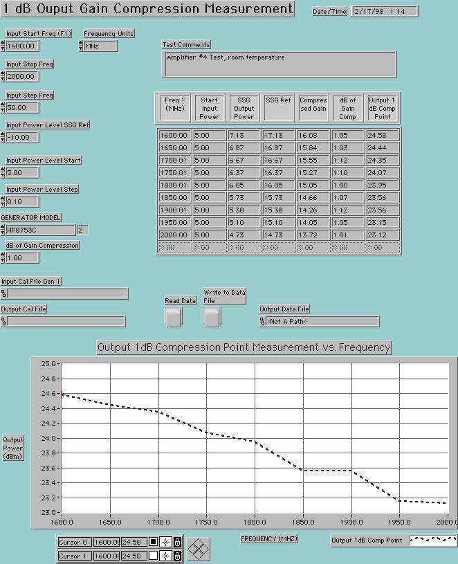
This LabVIEW panel shows the results of a computer automated 1 dB Output Gain Compression Point measurements for a PCS band RF amplifier. Measurements were performed using a programmable signal generator and a spectrum analyzer. A power meter was used to calibrate the input and output cables and connectors, and the spectrum analyzer amplitude readings. This panel design is tailored toward an "engineering evaluation" environment, instead of a "production test" environment. This is just one example of the types of automated RF measurements that can be performed using LabVIEW.

Computer Automated Noise Figure Measurements

LabVIEW Example - Computer Automated Noise Figure Measurements

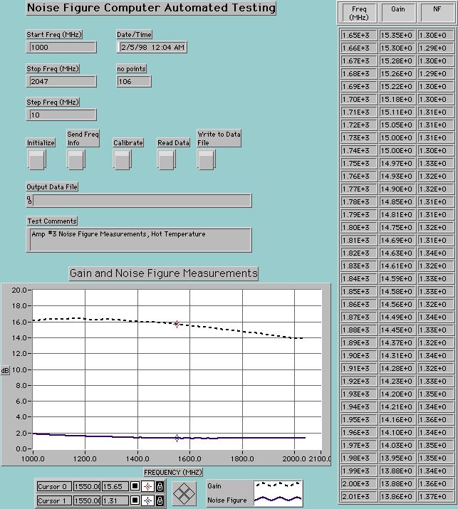
This LabVIEW panel shows the results of computer automated Noise Figure measurements for a PCS band RF amplifier. Measurements were performed using a HP-8970B Noise Figure Meter. This panel design is tailored toward an "engineering evaluation" environment, compared to a "production test" environment. This is just one example of the types of automated RF measurements that can be performed using LabVIEW.

Software Controlled Laser Power Meter Interface

Software Controlled Laser Power Meter Interface

• Software was developed to provide a computer-controlled interface to a Universal Radiometer. The Universal Radiometer is a piece of test equipment used to measure laser power. The device was controlled by a PC serial port. The software was developed using National Instruments LabVIEW graphical programming language.
• All instrument controls are sent from the screen display through the PC serial port to the test equipment.
• Data from the test equipment is sent via the PC serial port to the computer and analyzed and displayed on the screen display.
• Measured data can be stored to an external file in Microsoft Excel or other spreadsheet compatible format.
• Measurement statistics are calculated and displayed in real time

Instantaneous Frequency Measurement (IFM)

LabVIEW Example - Instantaneous Frequency Measurement (IFM)

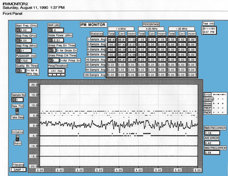
2. Explanation of Parameters on Data Plots

An explanation of the parameters on the data plots shown in Appendix A is provided below.

2.1. Start, Stop and Step Frequencies

Frequencies used for test data.

2.2. Noise Power (dBm)

The wideband noise power across the 2 to 6 GHz frequency band. The noise source was provided by cascading several 2-6 GHz amplifiers together and tuning the amps for flat gain across the frequency band. The noise power was measured using a broadband power meter.

In the NB filter measurements, the noise power represents the noise power across the NB filter bandwidth measured using a broadband power meter.

2.3. SNR

The Signal to Noise Ratio at the IFM input. The SNR was achieved by combining the signal and noise and adjusting the input RF signal relative to the wideband noise power measured.

2.4. Pulsewidth (nSec)

The pulsewidth of the IFM enable (Freq Strobe). The pulsewidth determines how many samples are received from the IFM at each frequency. There will be 1 frequency reading or average frequency output every 100 nSec over the IFM enable time

2.5. Data < 4 MHz

The percentage of frequency readings that were less than 4 MHz error were calculated. The readings were flagged correctly if the Gross Freq Error Flag was 0, and the PMOP Freq Error Flag was 0, and the Quality Bits were greater than or equal to the Quality Bit Threshold. The readings were flagged incorrectly if the Gross Freq Error Flag was 1, or the PMOP Freq Error Flag was 1, or the Quality Bits were less than the Quality Bit Threshold. Percentages of data flagged correctly and incorrectly were summarized.

2.6. Data 4 - 20 MHz

The percentage of frequency readings that were between 4 and 20 MHz error were calculated. The readings were flagged correctly if the Gross Freq Error Flag was 0, and the PMOP Freq Error Flag was 0, and the Quality Bits were less than the Quality Bit Threshold. The readings were flagged incorrectly if the Gross Freq Error Flag was 1, or the PMOP Freq Error Flag was 1, or the Quality Bits were greater than or equal to the Quality Bit Threshold. Percentages of data flagged correctly and incorrectly were summarized.

2.7. Data > 20 MHz

The percentage of frequency readings that were> 20 MHz error were calculated. The readings were flagged correctly if the Gross Freq Error Flag was 1, or the PMOP Freq Error Flag was 1. The readings were flagged incorrectly if the Gross Freq Error Flag was 0, and the PMOP Freq Error Flag was 0. Percentages of data flagged correctly and incorrectly were summarized.

2.8. Quality Bit Threshold

The three quality bits comparing the last two correlator channels is an output of the IFM with each frequency reading. A seven (111) represents high correlation, and 0 (000) represents poor correlation between the correlator channels. The quality bits were compared against the Quality Bit Threshold to flag frequency readings in the range 4 to 20 MHz error. If the quality bits were less than the Quality Bit Threshold, and the Gross Freq Error and PMOP Freq Error were at logic 0, then the data would be flagged as a fine frequency error (4 - 20 MHz).

2.9. Gross Freq Error Threshold

The Gross Freq Error Threshold was programmed as an input to the IFM. If the worst case of all the correlator compares in the IFM is less than the Gross Freq Error Threshold, then the Gross Freq Error Flag is set to logic 1. The Gross Freq Error Flag is used to flagged errors > 20 MHz. See Appendix B for further information.

2.10. Gross PMOP Count Threshold

The Gross PMOP Count Threshold represents the number of IFM samples where the PMOP flag was looked at to determine low SNR conditions. If the the PMOP Flag was logic 1 at or before the Gross PMOP Count Threshold (no. of samples), then the PMOP Freq Error Flag would be set to logic 1. The PMOP Freq Error Flag is used to flag errors > 20 MHz. See Appendix B for further information.

2.11. PMOP Threshold

The type of phase modulation being detected (90° / 180°).

2.12. Sample No.

The plot shows results for the Sample No. on the left side of the plot. Note: the software program starts all arrays with element "0". Therefore, Sample 0 corresponds to the first frequency reading, Sample 1 corresponds to the second frequency average, etc.

2.13. Data Plots

The data plots on each page show test results for the Sample No. shown. The top trace shows the Quality Bits for each frequency reading. a 7 (111) represents good quality and 0 (000) represents poor quality.

The second trace shows the frequency error across the frequency band (MHz)

The third trace shows the Gross Freq Error Flag for each frequency reading. The trace is offset at -5 for clarity. When the value is -5, the flag is logic 0. When the value is -4, the flag is logic 1.

The fourth trace is the PMOP Freq Error Flag. If the PMOP flag is logic 1 in less than the Gross PMOP Count Threshold sample no, the PMOP Freq Error Flag is set to Logic 1. This trace is offset at -10 for clarity.

The fifth trace is the FMOP Flag, offset at -15 for clarity.